

A question we get asked again and again is what is the difference between a FEM calculation and manual calculation.
Many users find it very difficult to understand how a FEM analysis works and how it should be checked/verified.
This article is intended to provide explanation and clarity.
To calculate statics, the equilibrium of forces is applied.
\Sum{  }{  }{ Fx = 0  }

\Sum{  }{  }{ Fy = 0  }

\Sum{  }{  }{ M = 0  }
For a simple system with multiple loads, the calculation is as follows.
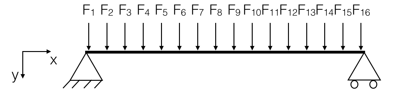
\Sum{ }{ }{ Fy = 0 => 0 = FA + FA + F1 + F2 + ... + F3 } \Sum{ }{ }{ MA = 0 => 0 = F2 * l / 16 + F2 * 2 * l / 16 + F3 * 3 * l / 16 + ... F16 * l + FB }
These calculations can be automated very easily, for example with an Excel table. The distance to one of the bearings is entered and you can easily calculate the forces at the bearings.
This system also works with line loads, where the length of the line loads must also be recorded.
The accuracy of the calculations then depends on how exactly the distances to the bearings are indicated. One can also control the calculation by recalculating by hand.
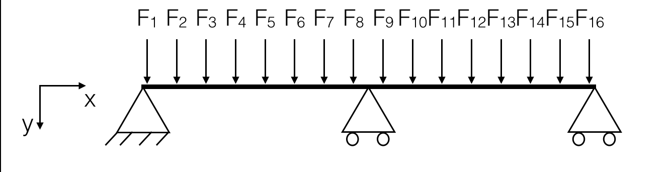
As long as statically determined systems are calculated, this approach can be applied. Statically determined systems are all systems with a maximum of two supports for line structures and three supports for spatial structures. More information about statically determined and indefinite system can be found here
For calculations of statically undetermined systems, this method does not work. Applying them inevitably leads to wrong results. To calculate such systems, you have to apply the differential equation of beam.
The differential equation on beam describes the interaction between acting forces and deformations.
It runs as follows:
E * I * w\left( x \right) = \Integ{ }{ }{ \Integ{ }{ }{ \Integ{ }{ }{ \Integ{ }{ }{ -dx } } } }
Whereby:
Since the whole thing is a function, it is only valid between two point loads. So in the case we have it above, we have 16 areas where we have to set up this function.
With the ... you can write down the formula as follows.
A manual calculation for such a system, by integration, is incredibly time-consuming and very error-prone. Every engineer does this once during his studies with a clearly simple system and then uses a different process.
Fortunately, there is the property that these systems can overlap.
The basic idea of the FEM method is to break down the structure to be calculated into a larger number of elements with easily manageable properties and then combine them into a complex system of equations while preserving the kinematic compatibility conditions and the static equilibrium conditions. (2 p. 87)
The support structure is discretized into so-called finite elements. These elements are connected only at nodes. At each node, the displacement variables and force quantities are defined.
The resulting system of equations has the basic form:
Stiffness x displacements = forces
Whereby the stiffness and the acting forces are known and thus the unknown displacement can be determined. The material law can be used to establish the connection between displacements and stresses. (3 p. 7)
The finite basic equation therefore has the following form:
𝑘∙𝑢=𝐹
k represents the existing elastic stiffness, u the unknown displacements and F the known forces.
One can also understand this form of equation also as a linear system of equations in the form
𝐴∙𝑥=𝑦
Here, A denotes a symmetric matrix, x the vector with the unknowns and y the vector with known results. This system of equations can now be solved with the Gauss algorithm or the Cholesky method8.
Basic procedure for FEM solutions according to (2 p. 90):
1. Determination of element stiffness matrices and node loads
2. Structure of the system stiffness matrix consisting of the element stiffness matrices and the load vector
3. Solution of the system of equations for the displacement variables
4. Determination of the support reactions from the displacement variables
5. Determination of the element stresses (internal forces) from the displacement variables
For the calculation of a truss corner, the individual rods are idealized as beams. Beams have the property that their cross-sectional dimensions are small compared to their length. (4 p. 89)
For a three-dimensional beam, the following properties are modeled for each node k:
| Deformation | Power |
|---|---|
| u𝐹 | Fxk |
| 𝒗𝐹 | Fyk |
| v𝐹 | Fzk |
| 𝝋x𝒌 | 𝑀x𝑘 |
| 𝝋y𝒌 | 𝑀y𝑘 |
| 𝝋z𝒌 | 𝑀z𝑘 |
These quantities correspond to the local element-coordinate system.
The element stiffness matrix is a positively defined, symmetric 12x12 matrix. When using elements of this type to model real components, the following assumptions must be fulfilled:
Pipe cross-sections, such as those used in the trusses, are not susceptible to arch force torsion.
In a calculation according to theory I. order, the assumption is made that deformations are small. Therefore, nonlinear stress increases from the simultaneous action of normal force and bending moment are not considered.
This effect can be taken into account in the FEM calculation via the calculation according to theory II. For example, the Delta-P method is used for this purpose. (2 p. 490)
By choosing the 3D beam as a FEM element, the beam properties of a truss corner of the cross-section can be examined. Local influences at the joints, such as welds or screw connections, are not taken into account. For further investigations, the cross-section could be modeled with 3D solid elements. With the help of these FEM elements, these properties could also be investigated.
Especially with large systems, a calculation of the system is often only possible via FEM. Manual calculation often only serves to feign better traceability.